My notes for MAT21C is incomplete since I regularly skip classes and only take notes on problems on the homework that I don’t know or forgot how to do from AP Calculus AB/BC.
Series
N: common Maclaurin series
common Maclaurin series
1−x1excosxsinxln(1+x)arctanx=n=0∑∞xn=n=0∑∞n!xn=n=0∑∞(2n)!(−1)nx2n=n=1∑∞(2n−1)!(−1)n−1x2n−1=n=1∑∞n(−1)n−1xn=n=1∑∞2n−1(−1)n−1x2n−1=1+x+x2+x3+…=1+x+2!x2+3!x3+…=1−2!x2+4!x4−6!x6+…=x−3!x3+5!x5−7!x7+…=x−2x2+3x3−4x4+…=x−3x3+5x5−7x7+…Link to original
P: binomial series expansion
binomial function Taylor series
We have a binomial function fm(x)=(1+x)m where m∈R.
If m is a positive integer, then the binomial function fm is a polynomial, and its Taylor series would be the same polynomial.
If m is not a positive integer, then its Taylor series has infinitely many non-zero terms. The Taylor series converges for ∣x∣<1 and is given by:
T(x)=1+n=1∑∞(nm)xn
with binomial coefficients (1m)=m, (2m)=2!m(m−1), and so on.
The dot product or scalar product of u and v is u⋅v. The resulting value is a scalar. The dot product is 0 when the vectors are orthogonal to each other.
A⋅B=ABcosϕ=∣A∣∣B∣cosϕ
length of A (or B) times the length of A (or B) in the direction of B (or A), a.k.a the length of the other side of the triangle
ϕ is the acute or flat angle between A and B
The dot product is equal to the sum of the product of the corresponding components. For example, if they are two dimensional, then:
u⋅v=ux⋅vx+uy⋅vy
# assume u, v are two tuples of arbitrary dimensionsassert len(u) == len(v)u_dot_v = sum([u_i * v_i for u_i, v_i in zip(u, v)])
find a parametric equation for the line where two planes intersect
Find normal vectors for the two plane.
![[normal vector#find—vecn-of-a-plane|Find vecn of a plane]]
The intersecting line has the same direction as n1×n2. Find the cross product.
NOTE: You don’t have to find the unit vector (direction) of the cross product, since the magnitude doesn’t matter, only the direction and where the initial point of the vector do (which we will determine later.
Find a point P shared by both planes where we can place the direction vector of the line.
find a point shared by two planes
Case 1: the point is apparent in the plane equations.
3(x+2)−2(y−1)+2(z+1)=0
(x+2)+2(y−1)−3(z+1)=0
Common point: (−2,1,−1)
Case 2: try setting one variable to zero, plug it into the plane equations, then solve the resulting system of equations (two equations, two variables). See this post.
Assume we are given four vertices A to D. Treat the A as the origin and calculate three vectors P=AB, Q=AC, and R=AD. These three vectors are the three edges ending on the same vertex. The volume is the triple scalar product of P, Q, and R, i.e., P⋅(Q×R), or find the determinant of their matrix from vertical concatenation).
P: intersection of lines or minimum distance between lines
intersection of lines or minimum distance between lines
Without already knowing if the lines intersect, we have to follow through these steps one by one.
Parallel - distance
First check whether the lines are parallel. The lines are parallel if the cross product of the direction vectors is zero. To find distance between parallel lines:
Find one point on each line. Let’s call them P and Q. Calculate the vector u=PQ
The distance d between the lines is
d=∣v∣∣u×v∣
where v is the direction vector for any one of the two lines.
Intersection?
If the lines aren’t parallel, we need to determine whether the lines intersect or are skew.
Treat the two parametric equations as a system of equations, and solve for both parameters. If the solutions are valid (check with all equations), then we have an intersection, otherwise the lines are skew. Detailed steps below:
Set the first pair of parametric equations (both x=⋯) equal to each other. Solve for one of the parameter (parametric variable).
Set the second pair of equations equal to each other. Plug the solved parameter in, and solve for the other parameter.
Set the third pair equal to each other. Plug the first parameter into it and solve for the other one. Check if the solution for the parametric variable is consistent with step 2. If not, then the lines are skew. If it is, then plug the one parameter into a line equation to obtain the intersection coordinate.
Skew!
To calculate distance between skew lines:
Find the cross product N between the two direction vectors. If the two lines were moved to the same plane, N would be its normal vector.
Then find any point on each line (P and Q) and calculate the vector PQ. Note that the N-component of PQ is the basically distance between these two lines. We can calculate that using projection.
The distance between the two lines is the projection of PQ onto N:
d=projNPQ=∣N∣PQ⋅N
The partial differentiation of an equation with respect to x (∂x∂) can be obtained by differentiating the equation with respect to x and treating other variables as if they were constants. For example, ∂x∂(3x+2xy)=3+2y .
For partial differentiation involving underlying variables, use chain rule and chain rule dependency diagram (e.g. ∂t∂y when y is defined not in terms of t, but some other variables that can be defined with t)
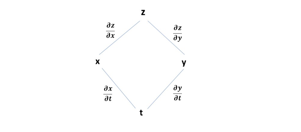
A chain rule dependency diagram is useful for calculating more involved partial differentiations using chain rule.
To draw a diagram for ∂t∂z, start from the initial function/variable, say z, which is defined in terms of undesired variables (say x and y). The diagram starts with z as the first node. Add the variables as children to the current variable’s node. Do this repeatedly to all the newly added child nodes (leaves) until they reach at the desired variable (t in this case). Each edge in the diagram represents a partial derivative (∂c∂p where p is the parent variable and c is child variable). For each possible path from the initial to the desired variable (z to t), multiply all the edges (e.g. z-x-t becomes ∂x∂z⋅∂t∂x). Sum all the paths together to get the desired partial differentiation (e.g. ∂t∂z=∂x∂z⋅∂t∂x+∂y∂z⋅∂t∂y).
Gradient of a multivariate function at a point is a vector pointing at the direction of steepest increase in value, with a magnitude of the function’s directional derivative in the pointed direction. each partial derivative. Its components consist of partial derivatives of the corresponding variables. For instance, ∇f(x,y,z)=∂x∂fi+∂y∂fj+∂z∂fk
P: find direction of maximum growth and decrease of function at point
find direction of maximum growth and decrease of function at point
At a point (a,b,c), the maximum growth is in the direction of the gradient (∣∇∣∇), and the maximum decrease is in the opposite direction (−∣∇∣∇). This can be used for optimization (e.g. stochastic gradient descent).
Assume the function z=f is defined in terms of x and y, i.e. z=f(x,y). Find the critical points (any minimum, maximum, or saddle point).
At critical points, fx=0 and fy=0, where f(⋅) is the partial derivative with respect to the corresponding variable. Solve the system of equations for x and y. Check the coordinates for extraneous solutions (not sure if this can happen but it might).
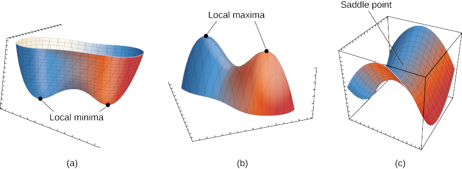
If f is a multivariate function, to determine whether z=f(x,y) has a minimum, maximum, or saddle point at the critical pointP=(x0,y0), we can use the second derivative test.
First find fxx, fyy, and fxy (fxx=∂x2∂2z, fxy=∂y2∂2f, fxy=∂x∂y∂2f). Then calculate the determinant D as below:
D=fxx(x0,y0)⋅fyy(x0,y0)−(fxy(x0,y0))2
Then:
If D>0 and fxx(x0,y0)>0, then f has a local minimum at P.
If D>0 and fxx(x0,y0)<0, then f has a local maximum at P.
P: evaluate a multivariate limit (or prove it doesn’t exist)
evaluate a multivariate limit
Try each step and move on to the next if indeterminate form is encountered:
Step 1 - Simple Substitution
Try just substituting the coordinate of the limit (x,y,…) into the expression.
Step 2 - Algebraic Manipulation
Factoring
If the expression is a fraction, try factoring the numerator and denominator and see if anything cancels. Then evaluate the limit again.
Multiply by conjugate over conjugate
If the fraction contains a root in numerator/denominator (e.g. in the form a+b), try getting rid of it by multiplying the fraction by the conjugate over conjugate. The conjugate for a+b is a−b. This might get rid of indeterminate forms if you are lucky.
Try to find other ways
See if there’s any other things you can try, like trignometry identities, to make the expression evaluatable.
Step 3 - Evaluate along paths to prove limit DNE
It’s likely that the limit does not exist, but we need to prove it. Try approaching the limit along different paths, like x=0 (y-axis), y=0 (x-axis), y=x, y=x3, etc. Substitute the value into the limit expression then evaluate the limit. If any two limits evaluated along different paths are not equal to each other, then the limit does not exist. Note that if two limits evaluated along different paths end up being equal, this number is not necessarily the limit of the function.
Level curves are like contour lines but for 3D functions.
To sketch level curves for a function, determine a range of z=f(x,y) values and step size (e.g. from -2 to 2 with step size 1, meaning c∈{−2,−1,0,1,2}). Then for each value of c: set c=f(x,y), solve for y, and draw the resulting curve.
For a (real) multivariate function (let’s say z=f(x,y)), its domain is a region R∈Rn where n is f‘s arity.
The boundary of R is a curve that separates points internal to the domain from the points outside the domain. Formally, a region in a plane is bounded if it lies inside a disk of finite radius. Note that boundary points can be either in or out of the domain, and two boundary points don’t have to all be in or out of the domain.
The domain is closed if R contains all boundary points, if any.
The domain is open if R contains no boundary points.
In cases where there is no boundary (e.g. when the domain is the entire plane), then the domain is both open and closed.
The domain can be neither open nor closed if R contains some but not all boundary points.
Given a piecewise function f:
f(x,y)={g(x)h(x)(x,y)=(0,0)(x,y)=(0,0)
Find its partial derivatives at every point (x,y)
For any point (x,y)=(0,0),
∂x∂f(x,y)∂y∂f(x,y)=∂x∂g(x,y)=∂y∂g(x,y)
Plug the y=0 into ∂x∂f, and evaluate. We need to check if the second derivative exists at this point. If not, then the partial derivative doesn’t exist at (0,0). Do the same for ∂y∂f.
If the second partial derivative does exist at (0,0) (piecewise is OK), and the left and right side first derivatives evaluate to the same value at (0,0), then the partial derivative exist at (0,0).
The dot product is equal to the sum of the product of the corresponding components. For example, if they are two dimensional, then: