What can be computed? a practical guide to the theory of computation

Metadata

• File: What can be computed by MacCormick (2018).pdf
• Zotero: View Item
• Type: Book
• Title: What can be computed? a practical guide to the theory of computation,
• Author: MacCormick, John;
• Publisher: Princeton University Press,
• Location: Princeton, New Jersey,
• Year: 2018
• ISBN: 978-0-691-17066-4

Abstract

Tags and Collections

• Keywords: 03 In Progress; ECS120

Comments

Annotations

Annotations(4/22/2024, 9:13:35 PM)

“4.5” (MacCormick, 2018, p. 63)

“In the practical view, we see the three main physical pieces of the Turing machine: the control unit,theread-write head,andthetape.The tape contains cells, and each cell can store a single symbol.” (MacCormick, 2018, p. 72)

(MacCormick, 2018, p. 74)

Turing machine definition**

(MacCormick, 2018, p. 75)

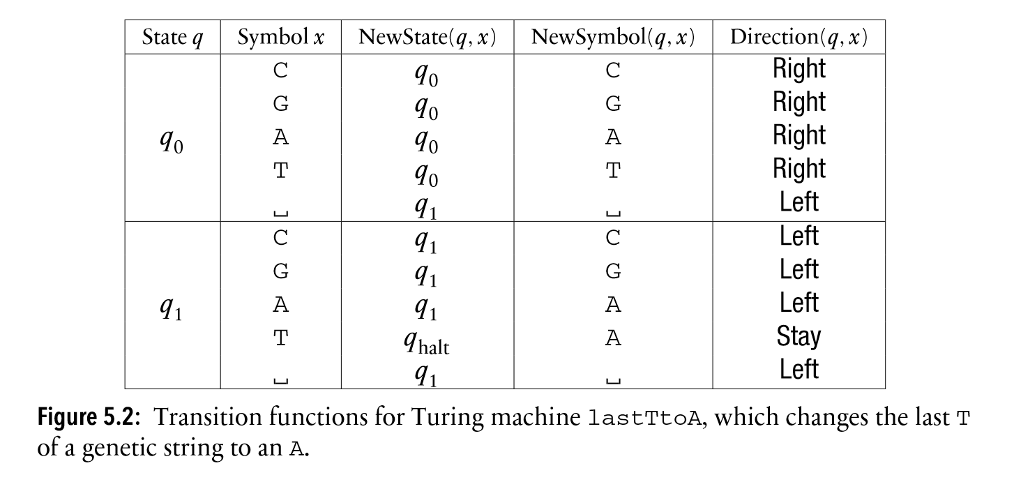
example machine lastTtoA (Turing machine project)**

(MacCormick, 2018, p. 76)

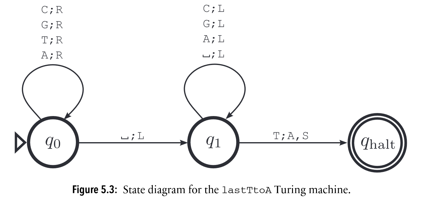
book’s convention for Turing machine state diagram**

“Sometimes, it’s convenient to think of a Turing machine as doing only one of these two tasks. If we are interested only in the output, the machine is called a transducer. If we are interested only in the accept/reject decision, the machine is called an accepter.” (MacCormick, 2018, p. 77)

(MacCormick, 2018, p. 78)

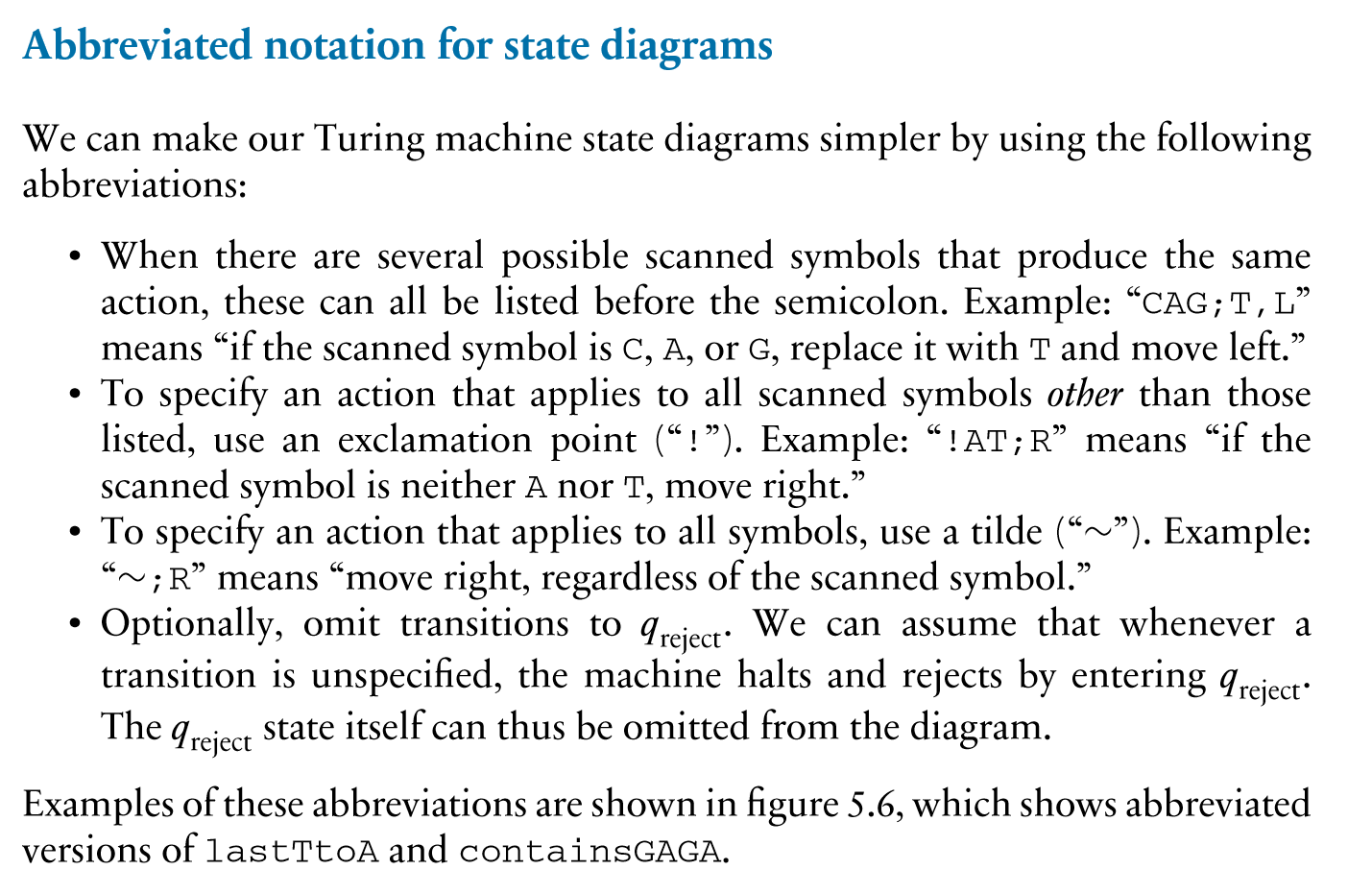
book’s convention for state diagram abbreviation**

“This final example demonstrates our convention that “xx” represents zero.” (MacCormick, 2018, p. 81)

“large, complex Turing machines can be built out of smaller, simpler blocks that are themselves” “Turing machines” (MacCormick, 2018, p. 82)

(MacCormick, 2018, p. 87)

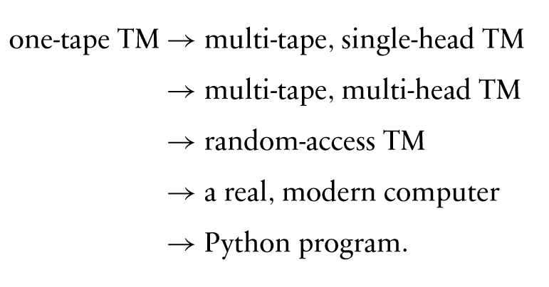
One-tape Turing machine can simulate a Python program.**

(MacCormick, 2018, p. 88)

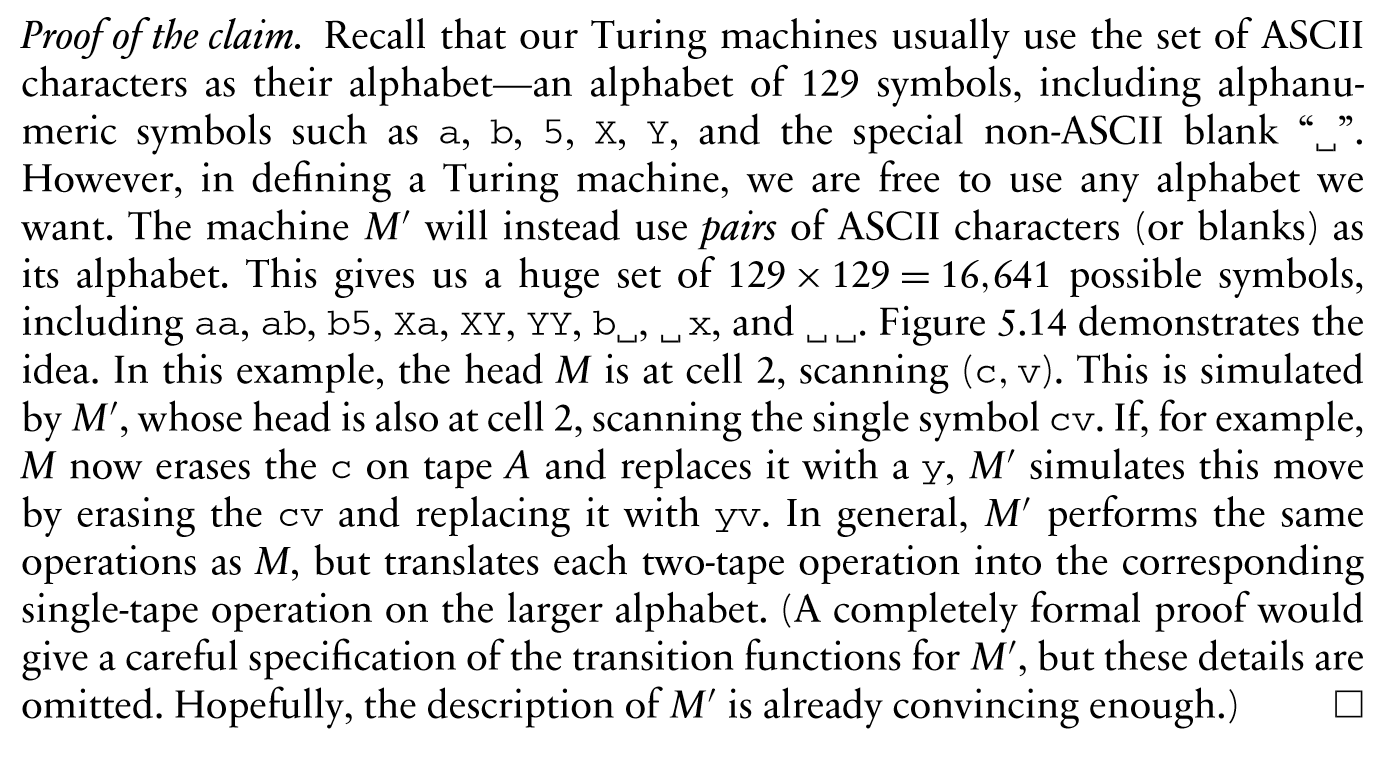
Proof: one-tape TM = two-tape TM in that we can combine a pair of symbols into a single symbol. That way, a two-tape TM is really the same as one-tape TM.**

“For example, to simulate a five-tape machine, we use an alphabet whose symbols consist of groups of five ASCII characters or blanks (like “x 2yz”). So, in terms of computability, a standard machine is just as powerful as any multi-tape, single-head machine.” (MacCormick, 2018, p. 89)

“Claim 5.2. Let M be a multi-tape, multi-head Turing machine. Then there exists a multi-tape, single-head Turing machine M′ that computes the same function as M. Proof of the claim. Initially, assume M has only two tapes, A and B (the generalization to more tapes will be obvious). Machine M′ will have four tapes: A1, A2, B1, B2, as shown in figure 5.16. Tapes A1 and B1 in M′ perform exactly the same roles as tapes A and B in M. Tapes A2 and B2 are used to keep track of where the head of M is on each of its tapes. Specifically, A2 and B2 are always” “completely blank except for a single “x” symbol in the cell corresponding to the head position of M. In figure 5.16, for example, M is configured with head A at cell 4, and with head B at cell 2. Machine M′ is simulating this configuration with an “x”atcell4ontapeA2 and at cell 2 on tape B2.Thereal head of machine M′ happens to be scanning cell 0. To simulate a step of M, the real head of M′ must sweep to the right from cell 0, searching for the x’s on tapes A2 and B2,andthen altering tapes A1 and B1 in the same way that M alters A and B. Again, we omit the detailed specification of the transition functions for M′.” (MacCormick, 2018, p. 91)

“It’s not hard to simulate a random-access Turing machine with a standard multi-tape machine. Each random access is simulated by running a small subprogram that counts the relevant number of cells from the left end of the RAM.” (MacCormick, 2018, p. 92)

(MacCormick, 2018, p. 94)

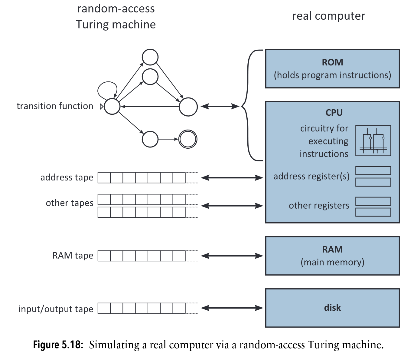
Random access TM simulates a real computer**

“Two computational models A and B are called Turing equivalent if they can solve the same set of problems. We say that A is weaker than B if the set of problems A can solve is a strict subset of the problems B can solve.” (MacCormick, 2018, p. 98)

“And there do exist stronger models of computation, but they are not physically realistic.” (MacCormick, 2018, p. 98)

Notes

Ch. 1: Introduction: What Can and Cannot Be Computed?

• tractable problems can be solved efficiently / in a reason amount of time
  • example: finding shortest route
  • Tractability has no precise definition, but it usually means polynomial time.
• intractable problems have solutions that are extremely expensive computationally
  • example: decrypt ciphertext without the key
  • superpolynomial time, exponential time, and beyond
• uncomputable problems cannot be computed by any program
  • example: find all bugs (crashes) in programs
  • These problems have been proved to be impossible to compute (e.g., produces a contradiction/paradox).
• computability theory studies the boundary between computable (tractable/intractable) and uncomputable problems
• complexity theorey studies the boundary between tractable and intractable problems

Ch. 2: What is a Computer Program?

• This book simplifies computer programs to single-file SISO (string-in string-out) Python programs, but this definition can be translated to any other programming language.
• book utils
  • rf(filename: str): str opens the given file and returns file contents as a string
• Assuming that Python programs are executed on the reference computer system $C$, a Python program is a string $P$ such that:
  • $P$ is syntactically correct Python.
  • $P$ has at least one function definition; when there is only one function definition, it must be the main function.
• The output $P(I)$ of a Python program $P$ on the reference computer system $C$ when $M$ is the main function:
  • $P(I)=S$ if $M$ returns an ASCII string $S$
  • $P(I)=\mathrm{undefined}$ if: $M$ returns an object that is non-ASCII string, $M$ throws an exception on $I$, or $M$ doesn’t terminate on $I$
• Assume the reference computer system $C$ can allocate as much memory as needed to execute the program.
• decision program: program that always outputs yes or no (unless undefined)
  • For a decision program $P$, $P$ accepts $I$ if $P(I)=\mathrm{yes}$, and $P$ rejects $I$ otherwise.
• Two programs are equivalent if $P_1(I)=P_2(I)$ for all possible inputs $I$.

Ch. 3: Some Impossible Python Programs

• review: proof by contradiction
• Consider that programs can use other programs (i.e., their source code)—and even themselves—as inputs.
• Consider the program $\text{yesOnString.py}(P,I)$ that returns “yes” if $P(I)=\mathrm{yes}$.
  • Let’s say there’s another program $\text{yesOnSelf.py}(P)$ that returns “yes” if $P(P)=\mathrm{yes}$.
  • Finally, consider the program $\text{notYesOnSelf.py}(P)$ that returns “yes” if $P(P)=\mathrm{no}$.
    • Note that $\text{notYesOnSelf.py}$ can be defined in terms of $\text{yesOnSelf.py}$, $\text{yesOnSelf.py}$ can be defined in terms of $\text{yesOnString.py}$.
    • Should $\text{notYesOnSelf.py}(\text{notYesOnSelf.py})$ return “yes” or “no”?
      • “yes”: Since it returns “yes” on self, the result should be “no”.
      • “no”: Since it returns “no” on self, the result should be “yes”.
      • $\text{notYesOnSelf.py}(P)$ is contradictory and thus cannot exist.
  • Since $\text{notYesOnSelf.py}$ is uncomputable, the programs $\text{yesOnString.py}$ and $\text{yesOnString.py}$, by which $\text{notYesOnSelf.py}$ could be written, must also be uncomputable.
• Consider $\text{crashOnString.py}(P,I)$ that returns “yes” if $P(I)$ crashes
  • Let there be $\text{crashOnSelf.py}(P)$ that returns “yes” if $P(P)$ crashes.
  • Finally, consider $\text{weirdCrashOnSelf.py}(P)$ that returns “yes” if $P(P)$ crashes, and crash otherwise.
    • This program can be written in terms of $\text{crashOnSelf.py}(P)$, which can in turn be written in terms of $\text{crashOnString.py}(P,I)$.
    • What’s the output of $\text{weirdCrashOnSelf.py}(\text{weirdCrashOnSelf.py})$?
      • returns “yes”: so it’s supposed to crash on self, but didn’t?
      • crash: it crashes on self, so it’s supposed to return yes?
  • Since $\text{weirdCrashOnSelf.py}$ program is contradictory, it cannot exist, and neither can the other two programs which can be used to write this program.

Ch. 4: What is a Computational Problem

• ”Programs solve problems.”
• graph terminology review
  • path: sequence of nodes connected by non-repeated edges
  • Hamilton cycle: path for which nodes traversed are unique except the starting and ending node which are the same
  • book’s convention for representing graph-related entities as strings:
    • path: comma-delimitted list of node labels
    • graph: space delimitted list of edges. each edge is a comma-delimitted pair of node labels, e.g., “a,b c,a b,d”
    • weighted graph: same as an unweighted graph, except each edge has an additional number (weight) appended to the end, e.g., “a,b,1 c,a,2 b,d,3”
  • tree
  • rooted tree (usually just called trees): a tree with a designated root node
• alphabet: a finite set of symbols
  • translation between alphabets: e.g., ASCII to binary (0/1)
  • An alphabet is usually denoted as $\Sigma$, e.g., a binary symbol can be denoted as $\Sigma =\left\{0,1\right\}$.
• string: finite sequence of zero or more characters from a given alphabet $\Sigma$
  • $ϵ$ denotes the empty string.
  • $st$ represents the concatenation of strings $s$ and $t$.
  • $s^k$ represents repetition of the string $s$, $k$ times.
• language / formal language: finite or infinite set of strings defined on a given alphabet
  • A language does not need to contain the empty string.
  • Any finite set of strings is a language.
  • $\varnothing$ and $\left\{\right\}$ denotes the empty language.
  • Convention: For any given alphabet $\Sigma$, the language formed by all strings on the alphabet is denoted ${\Sigma }^{\ast }$.
  • operations
    • union: $L_1\cup L_2$ (strings from either one or the other language)
    • intersection: $L_1\cap L_2$ (strings that are in both languages)
    • complement: $\overline{L}$ (strings in ${\Sigma }^{\ast }$ but not $L$)
    • concatenation: $L_1{L}_2$ (strings formed by concatenating $l_1$ and $l_2$)
    • repetition (Kleene star): $L^{\ast }$ (strings formed by repeating elements of $L$ zero or more times; does not need to repeat the same element)
• A computational problem is a function mapping strings on ${\Sigma }^{\ast }$ to sets of strings on ${\Sigma }^{\ast }$.
  • Each input to the problem may have multiple acceptable outputs (i.e., elements of the solution set).
  • Encoding/formatting of the input strings should not matter for any meaningful computational problem.
  • book’s convention
    • Assume that for invalid inputs, the solution set is always $\left\{\text{“no”}\right\}$.
    • Assume that when no solutions exist for the input, the solution set is always $\left\{\text{“no”}\right\}$.
    • The books will never use $f$ (function) and $P$ (program) to denote a computational problem.
• An input $s$ to the problem $F$ is called an instance of the problem.
  • An instance is negative if the $F(s)=\left\{\text{“no”}\right\}$ (i.e., no solution), positive otherwise.
• some types of computational problems
  • search problem: problems that involve finding a string $S$ for which $Q(I,S)$ is true given an input string $I$ and a predicate function $Q$ (or return “no” if $S$ does not exist).
  • optimization problem: problems that involve finding a string $S$ such that $V(I,S)$ be minimized (or maximized), given an input string $I$ and an objective function $V$ (numerical function).
    • This book only considers integer-valued numerical functions.
    • example: $\mathrm{ShortestPath}$ is an optimization problem where $V$ is the function outputting path length/cost, $I$ is the graph, and $S$ is the path.
  • threshold problem: problems that involve finding an $S$ such that $V(I,S)\le K$ given input $I$, threshold $K$, and a numerical function $V$. The conditions may be $\le$, $<$, $=$, etc.
  • function problem: problems whose solution sets are singletons (i.e., set of size one—each input has a unique solution).
  • decision problem: problems whose outputs are either “yes” or “no”.
    • Decision problems are elegant & handy when dealing with theory, but less useful in practice.
    • General computational problems refer to problems that are not decision problems
    • The complement $\overline{D}$ of a decision problem $D$ returns “no” whenever the decision problem returns “yes,” and vice versa.
• General computation problems often have a close decision problem counterpart (e.g., instead of asking “what is it?” like in the general computational problem, the decision problem variant asks “does it exist?” or “is it the right value?”).
• $P$ solves or computes a decision problem $F$ if $\forall I,P(I)\in F(I)$; if $F$ is a decision problem, then we can also say $P$ decides $F$. If $F$ can be computed, it is computable; if $P$ is a decision problem, we can also say it is decidable
• A language $L$ has an associated decision problem ${\mathrm{IsMember}}_L$ that decides if the input is a member of $L$. We can also define a language $L_D$ based on the set of strings accepted by a decision problem $D$.
  • Convention: To define a language for a multi-input decision problem $D$, use the format $L_D=\left\{ESS(A,B,\dots )|A(B,\dots )=\text{“yes”}\right\}$, where $ESS$ is a function from the book that stands for “Encode as Single String.”
• A program $P$ recognizes a language $L$ if for all inputs $I\in L$, $P(I)=\text{“yes”}$, and either $\text{“no”}$ or $\mathrm{undefined}$ otherwise. In other words, a recognizer must be able to say “yes” for positive instances (and “yes” for these only), but doesn’t need to halt for negative instances. Note that some undecidable languages can still be recognizable.
  • A decidable language $L$ is also recognizable, since $\mathrm{IsMembe}{\mathrm{r}}_{\mathrm{L}}$ can also be used to recognize the language.
• Side note: In earlier days of computation theory, decidable languages are called “recursive languages,” and recognizable languages are called “recursively enumerable” languages.

Ch. 5: Turing Machines: The Simpliest Computers

• Turing machines are mathematically abstracted versions of programs. All programs written in a Turing-complete programming language are equivalent to Turing machines, in that they can solve the same set of computational problems.
• Practically, a Turing machine consists of a control unit—a black box containing a program—that has a read-write head to interact with/move an infinite tape of symbols both ways (left and right).

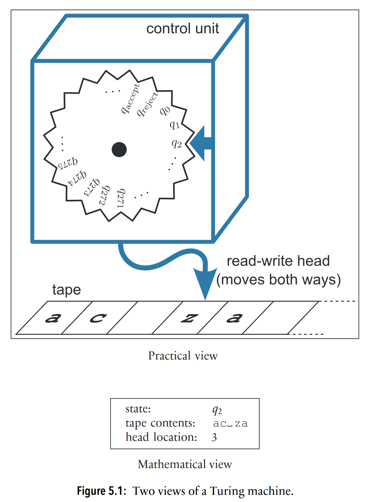
• The configuration is an exact description of a Turing machine at a moment in time, including its state, tape, and head position.
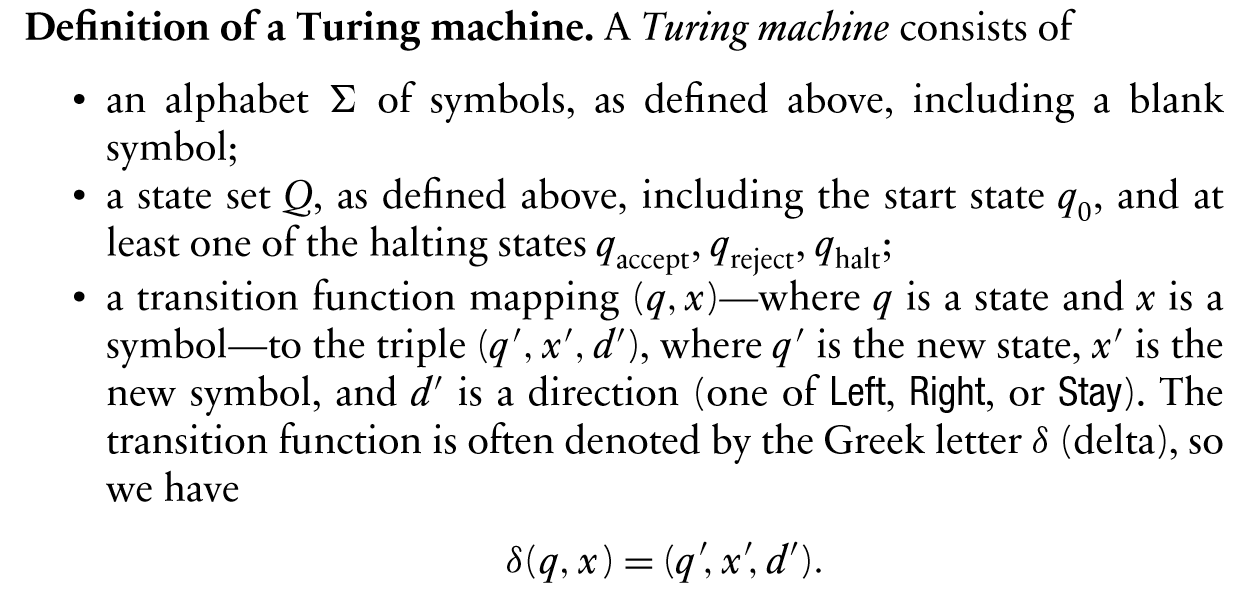
• Mathematically, a Turing machine is defined by five objects:
  • two sets
    • alphabet $\Sigma$: a finite set of symbols allowed on the tape, including the special blank symbol (uninitialized memory cell)
    • state set $Q$: finite set of machine states, including three special halting states: $q_{\mathrm{accept}}$, $q_{\mathrm{reject}}$, and $q_{\mathrm{halt}}$
  • three transition functions; alternatively, a mapping $(q,x)\to (q^{\prime },x^{\prime },d^{\prime })$
    • new state function: $q^{\prime }=\mathrm{NewState}(q,x)$ where $x$ is the scanned symbol (current symbol under read-write head)
    • new symbol function: $x^{\prime }=\mathrm{NewSymbol}(q,x)$
    • direction function: $d^{\prime }=\mathrm{Direction}(q,x)$
• Turing machine types (can be both)
  • transducer: output is useful to us
  • accepter: accept or reject state is useful to us
• The book uses a one-way infinite tape (the tape extends infinitely to the right).

Ch. 7: Turing Reduction

• If the computation problem $F$ has a Turing reduction to problem $G$, then $F$ can be solved if a program can solve $G$, and we can denote it with $F{\le }_{T}G$ ($F$ is as hard or less hard than $G$).
• techniques for proving a program to be uncomputable via Turing reduction
  • explain how an uncomputable program can be transformed into this program
  • write a Python program that transforms an uncomputable program’s supposed computation result into this program
  • use Rice’s theorem

Ch. 8

See annotations

Ch. 9: Finite Automata

A deterministic finite automata consists of:

• an alphabet $\Sigma$ that includes the blank symbol
• a state set $Q$ that must include start state $q_0$ and one of the halting states ($q_{accept}$, $q_{reject}$)
• transition function $\delta (q,x)\to q^{\prime }$, alternatively notated $\delta :Q\times \Sigma \to Q$. In each state, the machine consumes a character, moves the head to the right, and performs a state transition. The input tape has to be finite and cannot be modified. Since the tape only moves to the right, a dfa halts after at most $n$ steps.