MAT022A some lecture notes

2023-11-03 lecture 17

find particular solutions in presence of free variables

e.g.

$$\left[\begin{array}{ccc}1& -2& 1\\ 3& -6& 3\\ 4& -8& 4\end{array}\right]\cdot \left[\begin{array}{c}{x}_1\\ x_2\\ x_3\end{array}\right]=\left[\begin{array}{c}5\\ 15\\ 20\end{array}\right]$$

col vec 1, 2, 3 are multiples of each other. 2 free variables?

to find particular solutions, find augmented matrix

$$\left[\begin{array}{cccc}1& -2& 1& 5\\ 3& -6& 3& 15\\ 4& -8& 4& 20\end{array}\right]\to \left[\begin{array}{cccc}1& -2& 1& 5\\ 0& 0& 0& 0\\ 0& 0& 0& 0\end{array}\right]$$ $$x_1-2x_2+x_3=5$$

$x_2$ and $x_3$ are free variables, so set them to 0 to see that $x_1=5$

So this is a solution:

$$\left[\begin{array}{c}5\\ 0\\ 0\end{array}\right]$$

The problem is that how can we define the set of all solutions?

---

2023-11-05 lecture 18

$$\mathrm{span}\{\overline{v_1},\dots ,\overline{v_r}\}$$

How can we eliminate a redundant vector $\overline{v_i}$?

The set of vectors $\overline{v_1},\dots ,\overline{v_r}$ are linearly dependent if some $a_1\cdot \overline{v_1}+\cdots +a_r\cdot \overline{v_r}$ produces $\overline{0}$. Basically if some (if some coefficients are 0) or all vectors can cancel out, the set of vectors are linearly dependent. If all coefficients $a_i$ have to be zero to produce a zero vector, then the set of vectors are linearly independent.

The linearly dependent vector:

$$c_i\cdot \overline{v_i}=-c_1\cdot \overline{v_1}-\cdots -c_r\cdot \overline{v_r}$$

(right side doesn’t include $i$)

Columns of a vector are linearly indendent if null space is just the zero vector

---

2023-11-08 lecture 19

e.g.

Are these vectors linearly independent?

$$\left[\begin{array}{c}1\\ 2\\ 3\end{array}\right],\left[\begin{array}{c}0\\ 1\\ 1\end{array}\right],\left[\begin{array}{c}1\\ 0\\ 1\end{array}\right]$$

a.k.a. Is the null space of the matrix just zero vector?

$$\left[\begin{array}{ccc}1& 0& 1\\ 2& 1& 0\\ 3& 1& 1\end{array}\right]$$ $$\left[\begin{array}{ccc}1& 0& 1\\ 0& 1& -2\\ 0& 1& -2\end{array}\right]\to \left[\begin{array}{ccc}1& 0& 1\\ 0& 1& -2\\ 0& 0& 0\end{array}\right]$$

We use row operation to delete the third row (two rows are equal) → 3 vectors not linearly independent; one free variable $x_3$

For $x_3=1$ we have

$$\left[\begin{array}{c}-1\\ 2\\ 1\end{array}\right]$$

which is in the null space

e.g.

Are the columns LI? a.k.a. what’s the nullspace

$$\left[\begin{array}{cccc}1& 4& 7& 10\\ 2& 5& 8& 11\\ 3& 6& 9& 12\end{array}\right]$$

Since A is a 3 x 4 matrix, we can only have 3 pivots at most! So there is at least 1 free variable. (There can’t be 4 linearly independent vectors in 3D)

---

2023-11-13 lecture 20

• For a subspace V, dim(V) is the number of vectors in V’s basis.
• Basis vectors allow describing a vector $\overline{x}$ in the vector space as a linear combination of the basis vectors. The coefficients on the basis vectors are the coordinates of $\overline{x}$ in V in terms of those basis vectors.
  • Since all vectors in the basis are linearly independent, there is a unique set of coefficients for each vector $\overline{x}$.
    • Proof: Suppose there are two sets of coefficients $c$ and $d$. Then $(c_1-d_1)\cdot \overline{v_1}+\cdots +(c_r-d_r)\cdot {\overline{v}}_r=\overline{0}$
    • By the definition of linearly independence, the only solution to this equation is that all coefficient differences are 0 (the trivial solution). Thus $c_i=d_i$.
• Pivot columns of A (assume A is in rref) form a basis for $C(A)$. In other words, $\dim C(A)=\mathrm{rank}(A)$.
  • To show that basis vectors are linearly independent (which is already kind of obvious), show that the only possible linear combination of the basis vector that forms a zero vector is the trivial solution (all zero coefficients).
  • To show that the basis vectors span the column space of $A$, simply demonstrate that every column can be rewritten as the linear combination of basis vectors. This should be easy since pivot columns only have an element of 1 in separate row positions.

---

2023-11-15 lecture 21

• To identify columns of A as basis vectors when A is not in rref, simply turn A into rref and see which columns contain a pivot—the corresponding columns in the original A form a basis/are basis vectors.
  • Since we already know that $\mathrm{null}(A)=\mathrm{null}(\mathrm{rref}(A))$, we know that column’s linear independence (if any) remains the same when A is turned into rref, so we can safely use $\mathrm{rref}(A)$‘s pivot columns (LI) to identify basis vectors in A (also LI).
  • Generally, $\mathrm{C}(A)\ne \mathrm{C}(\mathrm{rref}(A))$, but $\dim (\mathrm{C}(A))=\dim (\mathrm{C}(\mathrm{rref}(A)))$. In other words, rref does not modify the dimension of the column space.
• To find a basis for $\mathrm{null}(A)=\mathrm{null}(\mathrm{rref}(A))$
  • The special solutions for Ax=0 where A contains free variables form a basis for null(A). Special solutions can be found by setting one free variable to 1 and other free variables to 0.
  • $\dim (\mathrm{Null}(A))=\text{number of free variables}$
  • Rank nullity theorem: Nullity = number of free variables = number of columns - rank = dim(Null(A))

---

2023-11-17 lecture 22

• To find the basis for the row space of a matrix
  • Row space of A is the column space of A transpose, since they use the same vectors. $\mathrm{R}(A)=\mathrm{C}(A^{\mathrm{T}})$
  • Row space does not change under row operations, so we can use rref to simplify A.
  • rref(A) gives us pivot rows. The pivot row vectors, when transposed to column vectors, form a basis for the row space.
• Equivalence
  • $\dim (\mathrm{R}(A))=\dim (\mathrm{C}(A^{\mathrm{T}}))=\text{number of pivots}=\mathrm{rank}(A)=\dim (\mathrm{C}(A))$
  • Note that generally $\mathrm{C}(A^{\mathrm{T}})\ne \mathrm{C}(A)$
    • e.g. $[12;00]$
• Projection
  • Given a $V\in {\mathbb{R}}^n$, $\overline{b}\in {\mathbb{R}}^n$ ($\overline{b}\notin V$ in general).
  • Projection of $\overline{b}$ onto $V$ is the closest approximation of $\overline{b}$ that still belongs in $V$.
  • $\overline{b}=\overline{c}+\overline{n}$ where $\overline{c}$ is the projection vector and $\overline{n}$ is a vector orthogonal to $V$.
  • For each $\overline{b}$, there is a unique $\overline{c}$ and $\overline{n}$.
    • Say ${\overline{c}}_1+{\overline{n}}_1=\overline{b}={\overline{c}}_2+{\overline{n}}_2$
    • It follows that ${\overline{c}}_1-{\overline{c}}_2={\overline{n}}_2-{\overline{n}}_1$
    • Left side is still in $V$, and right side is still a vector orthogonal to $V$, so $({\overline{c}}_1-{\overline{c}}_2)\cdot ({\overline{n}}_2-{\overline{n}}_1)=0$.
    • But since we know both factors are equal, we can rewrite it as $({\overline{n}}_2-{\overline{n}}_1)\cdot ({\overline{n}}_2-{\overline{n}}_1)=0$, which means ${\overline{n}}_1-{\overline{n}}_2=\overline{0}$. This means that there can only be one $\overline{n}$. The other factor involving $\overline{c}$ is also zero, so there can only be one $\overline{c}$.

---

2023-11-20 lecture 23

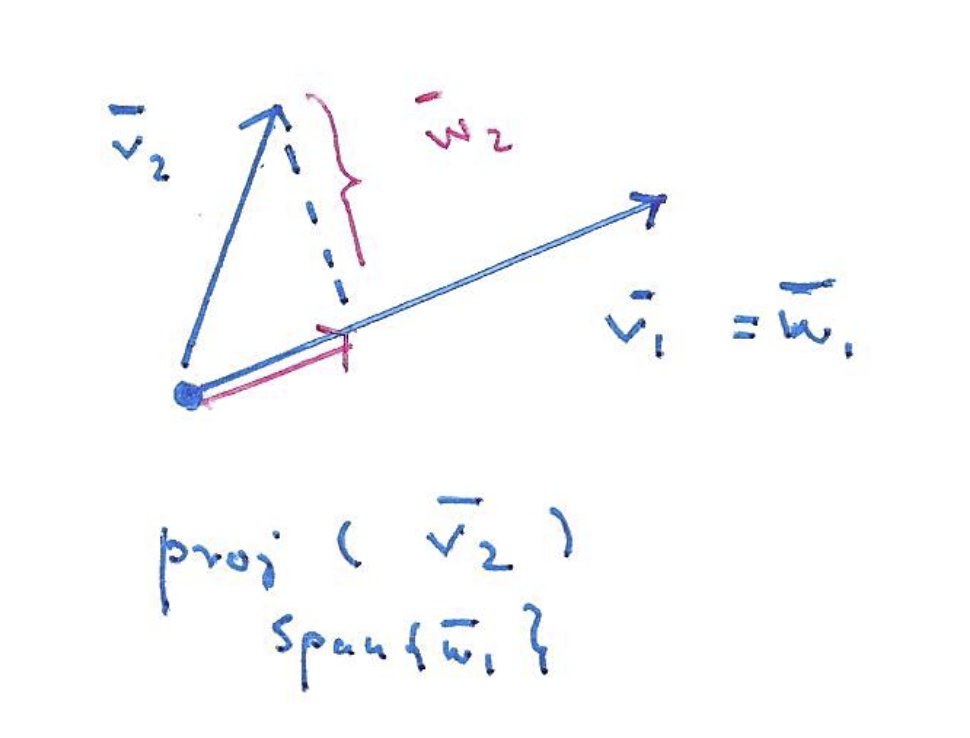
• To actually calculate $\overline{b}$‘s projection onto $V$, a.k.a. ${\mathrm{proj}}_V(\overline{b})$ assuming $V$ is aline
  • Say $V$ is a line, so $V=\mathrm{span}(\overline{a})$
  • ${\mathrm{proj}}_V(\overline{b})=\lambda \cdot \overline{a}$. We have to find this $\lambda$
  • We know $\overline{n}=\overline{b}-{\mathrm{proj}}_V(\overline{b})$. So $(\overline{b}-{\mathrm{proj}}_V(\overline{b}))\cdot \overline{a}=0$.
  • $(\overline{b}-\lambda \cdot \overline{a})\cdot \overline{a}=0$, so $\overline{b}\cdot \overline{a}-\lambda \cdot \overline{a}\cdot \overline{a}=0$
  • $\lambda \cdot \overline{a}\cdot \overline{a}=\overline{a}\cdot \overline{b}$
  • $\lambda =\frac{\overline{a}\cdot \overline{b}}{\overline{a}\cdot \overline{a}}$
  • So the projection of $\overline{b}$ onto $V$ (given a vector $\overline{a}$ that spans $V$) is $\frac{\overline{a}\cdot \overline{b}}{\overline{a}\cdot \overline{a}}\cdot \overline{a}$
  • If $\overline{a}$ is a unit vector, $\overline{a}\cdot \overline{a}=1$, so ${\mathrm{proj}}_V(\overline{b})=(\overline{a}\cdot \overline{b})\cdot \overline{a}$
• To find $\overline{b}$‘s projection onto $V=\mathrm{C}(A)$ for any matrix $A$
  • The projection can be described as ${\mathrm{proj}}_V(\overline{x})=P\cdot \overline{x}$ for some matrix $P$.
  • Condition 1: We know $P\cdot \overline{x}\in \mathrm{C}(A)$, so we know that $P\cdot \overline{x}=A\cdot \overline{y}$ for some $\overline{y}$.
  • Condition 2: We know $\overline{x}-P\cdot \overline{x}$ is orthogonal to $V$.
  • It follows from condition 2 that $A^{\mathrm{T}}\cdot (\overline{x}-P\cdot \overline{x})=\overline{0}$, since each row of $A^{\mathrm{T}}$ is a column of $A$, and since all columns of $A$ belong to the column space, the dot product of any column with the orthogonal vector will be zero, thus all elements of the product vector will be zero.
  • We can get $A^{\mathrm{T}}\cdot \overline{x}=A^{\mathrm{T}}\cdot P\cdot \overline{x}=A^{\mathrm{T}}\cdot A\cdot \overline{y}$ by distributing and then substituting in condition 1.
  • When $A^{\mathrm{T}}\cdot A$ has an inverse, we can use the leftmost and rightmost side to get $\overline{y}=(A^{\mathrm{T}}\cdot A{)}^{-1}\cdot A^{\mathrm{T}}\cdot \overline{x}$
  • Using the middle side, we get $P\cdot \overline{x}=A\cdot \overline{y}=A\cdot (A^{\mathrm{T}}\cdot A{)}^{-1}\cdot A^{\mathrm{T}}\cdot \overline{x}$
  • So we can use $P=A\cdot (A^{\mathrm{T}}\cdot A{)}^{-1}\cdot A^{\mathrm{T}}$ to project any vector onto $V$ via $P\cdot \overline{x}$.

---

2023-11-22 lecture 24

• Projection matrix $P$ is just an identity matrix without the pivots that are not needed to span $A$.
• Using $P$‘s definition, we can see that $P^2=P$.
• Using the projection matrix method, we can also find the projection of a vector onto a line (spanned by $\overline{a}$, so $A=\overline{a}$).
  • $P=A\cdot (A^{\mathrm{T}}\cdot A{)}^{-1}\cdot A^{\mathrm{T}}=\frac{1}{\overline{a}\cdot \overline{a}}\cdot A\cdot A^{\mathrm{T}}$
  • When $A=\overline{a}$, $P$ is a $2\times 2$ matrix with a rank of one since we’re projecting onto a line.
  • Is $(\overline{a}\cdot \overline{b})\cdot \overline{a}=P\cdot \overline{b}$? Yes.
    • Generally, $i$-th row of left-hand side is $\left({\sum }_{j=1}^n{a}_i\cdot b_i\right)\cdot a_i$ given $\overline{a}$ and $\overline{b}$ are column vectors with $n$ rows.
    • Generally, $i$-th row of right-hand side is $(\overline{a}\cdot {\overline{a}}^{\mathrm{T}}{)}_i\cdot \overline{b}=(a_i\cdot {\overline{a}}^{\mathrm{T}})\cdot \overline{b}=a_i\cdot \left(a_1\cdot b_1+\cdots +a_n\cdot b_n\right)=\left({\sum }_{j=1}^n{a}_i\cdot b_i\right)\cdot a_i$
    • Both sides are equal.

---

2023-11-27 lecture 25

• Projections can be useful for approximating a solution $A\cdot \overline{x}=\overline{b}$ when solution doens’t exist (e.g. estimate line of best fit).
  • Solution exists iff $\overline{b}\in \mathrm{C}(A)$
  • When solution doesn’t exist, we can find an approximate $\hat{x}$ such that $A\cdot \hat{x}$ is very close to $\overline{b}$.
  • least squares solution to $A\cdot \overline{x}=\overline{b}$: To approximate, solve $A\cdot \hat{x}={\mathrm{proj}}_{\mathrm{C}(A)}(\overline{b})$
    • Called least squares because the norm of a vector is defined as $\sqrt{d_1^2+\cdots +d_n^2}$
  • We have $A\cdot \hat{x}={\mathrm{proj}}_{\mathrm{C}(A)}(\overline{b})$
  • $A\cdot \hat{x}=\underset{\text{projection matrix}}{\underbrace{A\cdot (A^{\mathrm{T}}\cdot A{)}^{-1}\cdot A^{\mathrm{T}}}}\cdot \overline{b}$
  • $A^{\mathrm{T}}\cdot A\cdot \hat{x}=\underset{I}{\underbrace{A^{\mathrm{T}}\cdot A\cdot (A^{\mathrm{T}}\cdot A{)}^{-1}}}\cdot A^{\mathrm{T}}\cdot \overline{b}$
  • $A^{\mathrm{T}}\cdot A\cdot \hat{x}=A^{\mathrm{T}}\cdot \overline{b}$ (solve this equation to get least squares solution)

---

2023-11-29 lecture 26

• orthonormal basis: basis of a subspace $V\in {\mathbb{R}}^n$ where basis vectors are normal (size 1) and orthogonal to each other.
  • Formally, $\left\{{\overline{v}}_1,\dots ,{\overline{v}}_k\right\}$ is an orthonormal basis if ${\overline{v}}_i\cdot {\overline{v}}_j=0,\forall i\ne j$ (orthogonal) and ${\overline{v}}_i\cdot {\overline{v}}_i=1$ for all $i$ (normal).
  • Note that orthonormal bases are not unique for a subspace.
  • Orthonormal basis is useful for projections.
    • If $A$ has orthonormal columns, then $A^{\mathrm{T}}\cdot A=I$
    • $P=A\cdot \underset{I}{\underbrace{{\left(A^T\cdot A\right)}^{-1}}}\cdot A^{\mathrm{T}}$
    • $P=A\cdot A^{\mathrm{T}}$
• Gram-Schmidt algorithm: makes a basis (e.g. columns of matrix) orthonormal
  • Side note: If the basis vectors are already orthogonal, dividing each vector by their norm produces a orthonormal basis.
  • Observe that if $\left\{\overline{a},{\overline{b}}_1,\dots ,{\overline{b}}_k\right\}$ forms a basis for $V$, then so does $\left\{\overline{a}-\left({\sum }_{j=1}^k{c}_k\cdot {\overline{b}}_k\right),{\overline{b}}_1,\dots ,{\overline{b}}_k\right\}$.
    • This preserves linear independence since when we use the zero vector test, each subtracted term of $c_k\cdot {\overline{b}}_k$ can be distributed and grouped with the corresponding basis vector ${\overline{b}}_k$. All the coefficients still has to be zero for the linear combination to be the zero vector.
  • to be continued

---

2023-12-01 lecture 27

• Gram-Schmidt algorithm cont’d
  • Initial goal: Convert ${\overline{v}}_i$ (basis vectors of $V$) to ${\overline{w}}_i$, where (${\overline{w}}_i\cdot {\overline{w}}_j=0$, i.e. basis vectors are orthogonal). Normality can be achieved easily: divide the orthogonal vectors by norm.
  • Say there are 3 basis vectors without loss of generality
  • To start, we can make ${\overline{w}}_1={\overline{v}}_1$
  • To find a ${\overline{w}}_2$ orthogonal to ${\overline{w}}_1$, find ${\mathrm{proj}}_{{\overline{w}}_1}{\overline{v}}_2$. Then we can find a vector orthogonal to ${\overline{v}}_1$ via ${\overline{w}}_2={\overline{v}}_2-{\mathrm{proj}}_{{\overline{w}}_1}{\overline{v}}_2$.
    • 
    • Note that $\mathrm{span}\left\{{\overline{v}}_1,{\overline{v}}_2\right\}=\mathrm{span}\left\{{\overline{w}}_1,{\overline{w}}_2\right\}$
    • It can also be shown that ${\overline{w}}_2\cdot {\overline{w}}_1={\overline{w}}_2\cdot {\overline{v}}_1$.
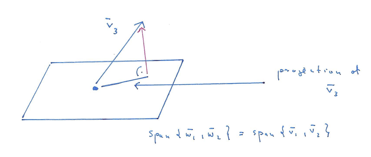
  • To find a ${\overline{w}}_3$ orthogonal to both ${\overline{w}}_1$ and ${\overline{w}}_2$, form a plane with both vectors and subtract the projection of ${\overline{v}}_3$ onto the plane from ${\overline{v}}_3$. In other words, ${\overline{w}}_3={\overline{v}}_3-{\mathrm{proj}}_{\mathrm{span}\left\{{\overline{w}}_1,{\overline{w}}_2\right\}}{\overline{v}}_3$. Note that projection onto the plane (with orthogonal basis vectors) can be split into projections onto ${\overline{w}}_1$ and ${\overline{w}}_2$ like so: ${\overline{w}}_3={\overline{v}}_3-\frac{{\overline{v}}_3\cdot {\overline{w}}_1}{{\overline{w}}_1\cdot {\overline{w}}_1}\cdot {\overline{w}}_1-\frac{{\overline{v}}_3\cdot {\overline{w}}_2}{{\overline{w}}_2\cdot {\overline{w}}_2}\cdot {\overline{w}}_2$.
    • 
  • If there were more basis vectors ${\overline{v}}_i$, calculate ${\overline{w}}_i={\overline{v}}_4-{\sum }_{j=1}^{j-1}\frac{{\overline{v}}_i\cdot {\overline{w}}_j}{{\overline{w}}_j\cdot {\overline{w}}_j}\cdot {\overline{w}}_j$

---

2023-12-04 lecture 28

• Determinant of a matrix $A$, denoted $\det (A)$
  • Only square matrices have a determinant.
  • If $\det (A)=0$, then $A$ is not invertible (i.e. $A$ is singular, and $\mathrm{Null}(A)$ is bigger than $\left\{\overline{0}\right\}$).
  • $\det I=1$ where $I$ is the identity matrix
  • Determinant is the linear function of each row, i.e. if one row was scaled by $c$, then the determinant will also be scaled by $c$.
• Calculating determinant
  • If a matrix $A$ can be transformed into upper triangular form via row operations (but without switching rows or scaling rows), then $\det (A)=c_1\cdot c_2\cdot \cdots \cdot c_n$ where $c$ represents the set of diagonal elements.
    • If switching rows is needed to transform into upper triangular matrix, then invert the sign of the final determinant. Switching rows an odd number of times also negates the original determinant (switching rows an even number of times does not affect the sign).
  • For any 2x2 matrix, $\det \left[\begin{array}{cc}a& b\\ c& d\end{array}\right]=ad-bc$.

---

2023-12-06 lecture 29

• Determinant is primarily a tool to check if $A$ is invertible.
  • If determinant is non-zero, then we know $A$ can be transformed into upper triangular form via row operations.
  • Instead of transforming A ourselves, we can calculate $\det A$ directly via the entries of A.
• cofactor expansion
  • The cofactor $C_{i,j}$ of $A$ is the determinant of a smaller matrix where the $i$-th row and $j$-th column of $A$ is removed. In addition, the cofactor needs to be negated if $i+j$ is odd. In other words, $C_{i,j}=(-1{)}^{i+j}\det (A(i|j))$.
  • To calculate $\det A$, choose a row or column with the most zeros and the greatest elements (this is to make manual calculation easier), iterate over each row or column element $A_{i,j}$, calculate $A_{i,j}\cdot C_{i,j}$, then sum them together.
    • If the cofactor matrix is not 2x2, repeat cofactor expansion recursively.
• Eigenvalue & eigenvector: $A\cdot \overline{v}=\lambda \overline{v}$
  • An eigenvector $\overline{x}$ of a square matrix $A$ is one such that $A\cdot \overline{x}$ doesn’t change its direction, but only scales it by $\lambda$, which is called the eigenvalue. Any vector $\overline{v}$ that has the same direction as $\overline{x}$ will also be scaled by the same $\lambda$, and thus is also a eigenvector. There can be multiple eigenvectors with different directions for each $A$. Note that eigenvalues can be negative.
  • An eigenvector in a 3D rotation transformation would represent its axis of rotation.

---

2023-12-08 lecture 30

• Finding eigenvalue & eigenvector
  • An easier way to think about solving this equation is to reframe it into $A\cdot \overline{v}=(\lambda I)\cdot \overline{v}$, which can be rewritten as $(A-\lambda I)\overline{v}=\overline{0}$. We need to make sure that $\det (A-\lambda I)=0$ because we want a non-zero $\overline{v}$ that will only be possible if that matrix is invertible & has a larger nullspace than $\left\{\overline{0}\right\}$.
  • We can find the set of all eigenvalues by solving $\det (A-\lambda I)=0$, which turns out to be a equation with degree $n$ whose variable is $\lambda$.
  • To find eigenvectors, solve for the nullspace of $A-\lambda I$ for each $\lambda$. Each $\lambda$ should result in a nullspace of $\mathrm{span}\left\{\overline{v}\right\}$.
  • The formula for Fibonacci numbers can actually be rewritten in linear algebra. $\left[\begin{array}{cc}0& 1\\ 1& 1\end{array}\right]\cdot \left[\begin{array}{c}{F}_{n-1}\\ F_n\end{array}\right]=\left[\begin{array}{c}{F}_n\\ F_{n+1}\end{array}\right]$. The closed-form formula for Fibonacci sequence actually uses the 2 eigenvalues of $A$.